Managing MIDI pitchbend messages

When designing a synthesizer or a sampler, how should you interpret MIDI pitchbend messages so that they’ll have the desired effect on your sound? First let’s review a few truisms about MIDI pitchbend messages.

1. A pitchbend message consists of three bytes: the status byte (which says “I’m a pitchbend message,” and which also tells what MIDI channel the message is on), the least significant data byte (you can think of this as the fine resolution information, because it contains the 7 least significant bits of the bend value), and the most significant data byte (you can think of this as the coarse resolution information, because it contains the 7 most significant bits of the bend value).

2. Some devices ignore the least significant byte (LSB), simply setting it to 0, and use only the most significant byte (MSB). To do so means having only 128 gradations of bend information (values 0-127 in the MSB). In your synthesizer there’s really no reason to ignore the LSB. If it’s always 0, you’ll still have 128 equally spaced values, based on the MSB alone.

3. Remember that all MIDI data bytes have their first (most significant) bit clear (0), so it’s really only the other 7 bits that contain useful information. Thus each data byte has a useful range from 0 to 127. In the pitchbend message, we combine the two bytes (the LSB and the MSB) to make a single 14-bit value that has a range from 0 to 16,383. We do that by bit-shifting the MSB 7 bits to the left and combining that with the LSB using a bitwise OR operation (or by addition). So, for example, if we receive a MIDI message “224 120 95” that means “pitchbend on channel 1 with a coarse setting of 95 and a fine resolution of 120 (i.e., 120/128 of the way from 95 to 96)”. If we bit-shift 95 (binary 1011111) to the left by 7 bits we get 12,160 (binary 10111110000000), and if we then combine that with the LSB value 120 (binary 1111000) by a bitwise OR or by addition, we get 12,280 (binary 10111111111000).

4. The MIDI protocol specifies that a pitchbend value of 8192 (MSB of 64 and LSB of 0) means no bend. Thus, on the scale from 0 to 16,383, a value of 0 means maximum downward bend, 8,192 means no bend, and 16,383 means maximum upward bend. Almost all pitchbend wheels on MIDI controllers use a spring mechanism that has the dual function of a) providing tactile resistance feedback as one moves the wheel away from its centered position and b) snapping the wheel quickly back to its centered position when it’s not being manipulated.

5. The amount of alteration in pitch caused by the pitchbend value is determined by the receiving device (i.e., the synthesizer or sampler). A standard setting is variation by + or – 2 semitones. (For example, the note C could be bent as low as Bb or as high as D.) Most synthesizers provide some way (often buried rather deep in some submenu of its user interface) to change the range of pitchbend to be + or – some other number of semitones.

So, to manage the pitchbend data and use it to alter the pitch of a tone in a synthesizer we need to do the following steps.
1. Combine the MSB and LSB to get a 14-bit value.
2. Map that value (which will be in the range 0 to 16,383) to reside in the range -1 to 1.
3. Multiply that by the number of semitones in the ± bend range.
4. Divide that by 12 (the number of equal-tempered semitones in an octave) and use the result as the exponent of 2 to get the pitchbend factor (the value by which we will multiply the base frequency of the tone or the playback rate of the sample).

A pitchbend value of 8,192 (MSB 64 and LSB 0) will mean 0 bend, producing a pitchbend factor of 2(0/12) which is 1; multiplying by that factor will cause no change in frequency. Using the example message from above, a pitchbend of 12,280 will be an upward bend of 4,088/8191=0.499. That is, 12,280 is 4,088 greater than 8,192, so it’s about 0.499 of the way from no bend (8,192) to maximum upward bend (16,383). Thus, if we assume a pitchbend range setting of ± 2 semitones, the amount of pitch bend would be about 0.998 semitones, so the frequency scaling factor will be 2(0.998/12), which is about 1.059. You would multiply that factor by the fundamental frequency of the tone being produced by your synthesizer to get the instantaneous frequency of the note. Or, if you’re making a sampling synthesizer, you would use that factor to alter the desired playback rate of the sample.

See a demonstration of this process in the provided example “Using MIDI pitchbend data in MSP“. The process is also demonstrated in MSP Tutorial 18: “Mapping MIDI to MSP“.

Using MIDI pitchbend data in MSP

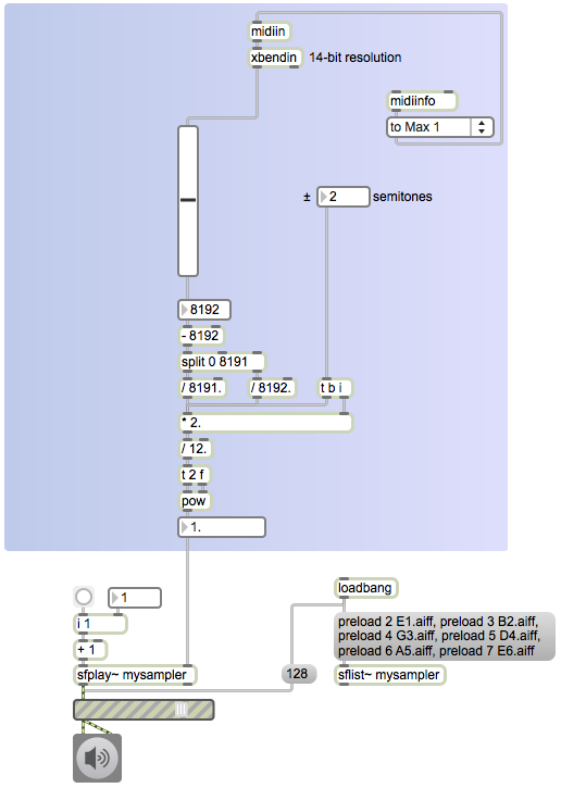
This Max patch demonstrates the arithmetic process of converting a MIDI pitchbend message into a factor that can be used to scale the fundamental frequency of a synthesized tone or the playback rate of a prerecorded sample in MSP.

The bendin object uses only the most significant byte (MSB) of the pitchbend message and outputs it as a value from 0 to 127. To get the full 14-bit resolution of an incoming message, one needs to use the midiin object to get the raw MIDI bytes, and then use the xbendin object to recognize pitchbend messages in the data stream, parse those messages, and combine the two data bytes into a single 14-bit value from 0 to 16,383.

A pitchbend value of 8192 (or of 64 if one is considering only the MSB) is considered the central value meaning no change in pitch. But it’s not literally exactly in the center of the range from 0 to 16,383, so in order to map the range 0-16,383 into the range -1 to +1 with 8192 in the center with a value of 0, one needs to treat the values below 8192 differently from the values above 8192. We do this by subtracting 8192 from the value so that the values now occupy the range -8192 to 8191, and then splitting the pitchbend values into two ranges and scaling the negative numbers by 1/8192 and the nonnegative numbers by 1/8191.

Once the values have been mapped into the range -1 to 1, they’re multiplied by the range of semitones desired (a range of ± 2 semitones is the norm). That number is then divided by 12 (the number of equal-tempered semitones in an octave) and that result is used as the exponent of 2 to get the frequency-scaling factor—the value by which we multiply the base frequency of the tone or the playback rate of the sample.


pitchbender.maxpat

For this patch to work correctly, you must download the six guitar string samples and save the decompressed sound files in the same directory as you save this Max patch.

In this example, we use the frequency-scaling factor to alter the playback rate of a prerecorded note. The sfplay~ object accesses a set of six preloaded sound cues, numbered 2 through 7. Each sound is a single guitar note, played at its original recorded rate. Since a playback rate of 1 gives the original pitch of the note, we can use the scaling factor directly to determine the desired playback rate for the “bent” note.

There are a few other things in this Max patch that bear explanation. Although they’re hidden from view, there are some objects in the patch that are included to make the slider object return quickly to its centered position the way that a real springloaded pitchbend wheel would do. On the left side of the patch there’s a demonstration of the same technique using the 7-bit pitchbend value from a bendin object. The right side of the patch demonstrates that an xbendin2 object will provide the two data bytes of each pitchbend message as two separate 7-bit values, and the patch demonstrates explicitly the bit-shifting and bit-masking operations that take place internally in the xbendin object to make a single 14-bit value.

Music 147 assignment for Tuesday April 29, 2014

To review the topic of sampling synthesis that we discussed in class, read the sections from Puckette’s The Theory and Technique of Electronic Music that deal with the topic of Wavetables and Samplers, including four of its first five subsections: The Wavetable Oscillator, Sampling, Enveloping Samplers, (you may skip the subsection on Timbre Stretching,) and Interpolation.

Study the API provided by either Java (Oracle) or Apple or Microsoft for assisting the programming of audio and music applications. In Java it’s known as the Java Sound API. In the MacOS and iOS it’s known as Core Audio. In Windows it’s the Core Audio APIs. In this class we will focus primarily on Java for cross-platform development and Objective C for MacOS/iOS development. Choose whichever is most familiar and useful to you, and teach yourself as much as possible about how basic audio functionality is handled, especially audio file I/O and audio stream I/O. Try to write a simple program that performs a basic I/O task such as a) opening and examining a file, b) generating a sound and playing it or storing it, c) copying input to output, etc.

Most importantly, come to class prepared to give a presentation on what you learned, and to engage in a discussion with others about best practices for basic audio programming with Java and/or Objective C. You’ll be called on to lead the class for at least a few minutes teaching something you know, or at the least, asking informed questions of others regarding what you don’t know.

Music 147 assignment for Thursday April 24, 2014

Keep working on your simple MIDI synthesizer. If you have not yet got it working to your satisfaction, make the modifications necessary to get it working, and resubmit it to the EEE DropBox folder “SimpleSynth1”. If you did already successfully complete the assignment, see if you can improve it by adding some additional functionality or some means of expressive control via MIDI. For example, you could try to implement pitch bending using MIDI pitchbend messages, or use the modulation wheel data—continuous controller number 1—to alter vibrato depth, tremolo depth (or rate), filter cutoff frequency, etc.

Music 147 lecture notes from Thursday April 17, 2014

1. We took a look at the project assignments as done by Brian MacIntosh, Jane Pham, Jared Leung, and Vanessa Yau. Brian’s solution played four simultaneous pseudo-random algorithmically-composed sinusoids. We discussed ways to avoid clicks when changing the frequency of a tone. Jane’s solution plotted the sum of two sinusoids. We identified a bug that was causing misrepresentation of the waveform. Jared’s program plotted and played a sinusoid and provided a slider for the user to select the desired frequency. We discussed interface choices and possible improvements, and discussed ways to schedule sound events so as not to interfere with simultaneous user events. Vanessa’s solution plotted the sum of three sinusoids. We discussed monitoring the sum of added sounds in the computer to avoid clipping, and we observed the difficulty of plotting a realtime sound stream when the fundamental period of the sound wave doesn’t correspond to the dimensions of the plot and the drawing rate of the program.

2. We discussed the concept of a “control function”, a function or shape that not heard directly but is perceptible because of the way it is used to affect change in a sound event.

For example, in the formula
f[n] = Acos(2π(ƒn/R+))
what if A, instead of being a constant value were a constantly changing value obtained from some other time-varying function of n? For example, it could be a linear function increasing from 0 to 1 (which would be a fade-in). Or it could be the output of a second oscillator function at a sub-audio frequency, which would result in a tremolo effect.

Control functions are important for giving shape and interest to an otherwise static sound, and also can be used to give shape to the musical content of the sound.

We built an example in Max in which we used a low-frequency oscillator (LFO) to modulate the frequency input of an audio-frequency oscillator, creating a vibrato effect. We discussed how the rate and depth of the frequency modulation affect the sound.

3. We went over the readings, and the examples of linear interpolation. We built an example in Max that uses the line~ object to create a breakpoint line segment function controlling the amplitude of a sound. In effect, we made four line segments that describe an attack-decay-sustain-release (ADSR) amplitude envelope emulating a note played by an instrument. We also used line~ to make a linear frequency glissando.

4. We discussed the math of linear interpolation.

The purpose of linear interpolation is to find intermediate values that lie on a straight line between two known values.

The underlying concept is:
To find intermediate y values that theoretically lie in between the y values at two successive x indices, as x progresses from one index to the next, intermediate y values can be estimated to lie on a straight line between the two known y values.

In other words:
If the y value at point x1 is y1, and the y value at point x2 is y2, then as x progresses linearly from x1 to x2, y progresses linearly from y1 to y2.

In other words:
The current value of y is to the range of possible y values as the current value of x is to the range of possible x values.

In other words:
(y-y1)/(y2-y1) = (x-x1)(x2-x1)
and
(y-y1)/(x-x1) = (y2-y1)/(x2-x1)

The general linear mapping equation to map one range of x indices to a corresponding range of y values is:
y = ((x-x1)/(x2-x1))*(y2-y1)+y1

This is applicable in discrete sampling terms because when we want to interpolate linearly from one value to another (say, from y1 to y2) over a series of samples (say, from na to nb), that implies that there will be b-a steps (increments) to get from y1 in sample na to y2 in sample nb.

So at each successive sample we would increase the value of y by (1/(b-a))*(y2-y1).

This interpolation algorithm is used for achieving a weighted balance of two signals.
Suppose we want a blend (mix) of two sounds, and we would like to be able to specify the balance between the two as a value from 0 to 1, where a balance value of 0 means we get only the first sound, a balance value of 1 means we get only the second sound, and 0.5 means we get an equal mix of the two sounds.

One way to calculate this is
y[n] = x1[n](balance)+x2[n](1-balance)
where x1 and x2 are the two signal values and balance is the weighting value described above.

Another way to calculate the same thing (slightly more efficiently) is
y[n] = x1[n]+balance(x2[n]-x1[n])
This second way involve one fewer multiplication than the first way.

When accessing a buffer of sample values or a ring buffer delay line or a wavetable array, for values of the index n that would fall between integer indices
(i.e. where n would have a factional part) we use the samples on either side of n—we’ll call them n0 and n1—and take a weighted average of the two.

One way to calculate this is
x[n] = x[n1](fraction)+x[n0](1-fraction)
where fraction is the fractional part of n.

Another way to calculate the same thing (slightly more efficiently) is
x[n] = x[n0]+fraction(x[n1]-x[n0])

5. We showed how the line~ object takes care of all that calculation for you in MSP, and allows you just to specify a destination value and a transition time to get there (or you can provide a series of such pairs: value and time.

Fade-ins and fade-outs, and multistep breakpoint line-segment functions (such as ADSR envelope shapes) can be easily generated by line~ (or adsr~), and can be drawn in the function object which then provides instructions to line~. You can apply these ideas to frequency as well as amplitude.

6. We discussed the logarithmic nature of our perceptions, as addressed in the Weber-Fechner law and in Stevens’ power law. I gave examples in both amplitude (loudness perception) in frequency (pitch perception). In an upcoming class I’ll explain tunings systems and equal temperament.

Mix two signals (more efficiently)

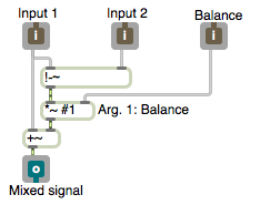
This demonstrates a linear interpolation formula for achieving a weighted balance of two signals. It has the exact same effect as the previous mixing example, but uses a more efficient formula, requiring one fewer multiplication per sample.

We want a blend (mix) of two sounds, and we specify the balance between the two as a value from 0 to 1, where a balance value of 0 means we get only the first sound, a balance value of 1 means we get only the second sound, and 0.5 means we get an equal mix of the two sounds.

The way we calculate this is
y[n] = x1[n]+balance(x2[n]-x1[n])
where x1 and x2 are the two signal values and balance is the weighting value described above.


mix2~.maxpat

The two audio signals come in the first two inlets, and the balance value comes in the right inlet. The argument #1 will be replaced by whatever is typed in as the object’s first argument when it’s created in the parent patch. This patch subtracts the sound coming in the first inlet from the sound coming in the second inlet, multiplies the result by balance and adds that result to the first sound.

A linear signal from 0 to 1 or from 1 to 0 coming in the right inlet will make a smooth linear crossfade between the two audio signals.

Mix two signals

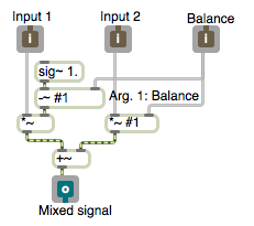
This demonstrates a linear interpolation algorithm used for achieving a weighted balance of two signals.

Suppose we want a blend (mix) of two sounds, and we would like to be able to specify the balance between the two as a value from 0 to 1, where a balance value of 0 means we get only the first sound, a balance value of 1 means we get only the second sound, and 0.5 means we get an equal mix of the two sounds.

One way to calculate this is
y[n] = x2[n](balance)+x1[n](1-balance)
where x1 and x2 are the two signal values and balance is the weighting value described above.


mix~.maxpat

In this MSP patch (abstraction), the two audio signals come in the first two inlets, and the balance value comes in the right inlet. Note the use of the argument #1, which will be replaced by whatever is typed in as the object’s first argument when it’s created in the parent patch. That allows the programmer to specify an initial balance value when using this abstraction. If the programmer doesn’t type in any argument, the #1 is replaced by 0, by default. The sig~ object provides a constant signal value. So this patch multiplies the sound coming in the first inlet by 1-balance, and it multiplies the sound coming in the second inlet by balance, then adds the two.

If, in the parent patch, the signal in the right inlet is a line~ object going from 0 to 1, the effect will be a linear crossfade between the sound in the first inlet and the sound in the second inlet.

Linear control function

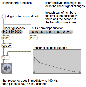
The line~ object generates a signal that interpolates linearly from its current value to a new destination value in a specified amount of time. It receives messages specifying a new value and the amount of time (in milliseconds) in which to get there. If it receives only a single number in its left inlet, it goes to that new value immediately.

We don’t listen to this signal directly (it’s not repetitive, so it’s not audible) but we perceive its effect when it’s used as a control function to change some parameter of a sound-generating algorithm.


lineardemo.maxpat

Note that a comma (,) in a message box enables you to trigger a series of messages by a single event. In effect, the comma means “End this message and follow it immediately by the next message.” So the message ‘440, 880 2000’ is actually two messages, ‘int 440’ and ‘list 880 2000’. It causes the linear signal to leap immediately to 440 and then transition linearly to 880 in 2000 milliseconds.

When the button is clicked, it triggers messages to both line~ objects. Over the course of 2 seconds, the amplitude is shaped by an ADSR envelope function, and the frequency sweeps from 440 Hz to 880 Hz, resulting in a 2-second note that glides from 440 Hz (the pitch A) to 880 Hz (the A above it).