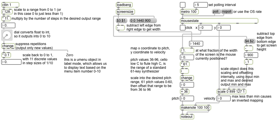
To translate numbers that occupy a particular range into an equivalent set of numbers in a different range, one common and useful technique is “linear mapping”. The term “mapping” refers to making conceptual connections between elements of one domain and elements of another, and “linear” mapping refers to using a mapping function that is a straight line–that is, such that numbers in one domain are mapped to an exactly equivalent position in the new domain. This is a very common and useful operation in media programming.

To do such a mapping requires the following operations. First, scale the range of the input values to occupy the desired range of outputs. The scaling operation is done by multiplication. An example of this would be if you want to map numbers that range from 0 to 127 (128 discrete integer values) into the range from 0 to 1); you could simply multiply all the input values by 1/127 (i.e., 1/(maximum-minimum) of the input range), which would result in outputs ranging from 0 to 1 in increments of 1/127, i.e., steps of size 0.007874. Then, if the entire output range needs to be adjusted upward or downward, you can offset the output by a certain amount. The offsetting operation is done by addition.

When the input range is divided up into a specific number of possible values, as is the case with integers 0 to 127 where there are 128 discrete possibilities, you might in some cases want to change the number of steps in the output range. In the example above, we had 128 discrete input values and wanted to map that onto the output range 0 to 1; but suppose we wanted the output to be only one of 11 discrete values, from 0 to 1 in increments of 1/10 (0.0, 0.1, 0.2, 0.3, … 1.0). We can multiply by the desired number of output values by 11 (the desired number of possible outputs) and divide by 128 (the number of possible inputs), convert those values to integers (by truncating the fractional part of the number), then scale that new range to the desired range by the method described in the previous paragraph (and finally adding an offset if necessary).

That’s what we did in the example on the left side of the patch. We take MIDI controller values from the mod wheel of a synthesizer (controller number 1, with 128 possible data values from 0 to 127), divide by 128 (the total number of possible inputs), multiply by 11 (the number of steps we want in our output range), convert the numbers to integers (the dial object does that for us internally by changing the data type from float to int), filtering out repetitions (the change object does that), resulting in 11 possible output values 0 to 10. To scale the range 0-10 down to the range 0-1, we multiply by 1/(maximum-minimum), which is to say 1/(10-0), which is 1/10, which is 0.1. That gives us 11 possible numbers ranging from 0 to 1 in ten equal steps.

Optionally you could re-scale that to any other size range (for example, multiply it by 100, which would give you a range from 0 to 100 in ten equal steps) and/or offset it by some amount. (for example, after multiplying by 100 you could add -50, which would give you a range from -50 to 50 in ten steps, i.e., -50, -40, -30, … 50).

On the right side of the patch, we use the cursor (mouse) coordinates on the screen to control the pitch and velocity of MIDI notes. First we get the dimensions of the screen, using the screensize object. It outputs the left, top, right, and bottom coordinates of the screen. By subtracting left from right, and top from bottom, we obtain the width and height of the screen, in pixels. Those are our input ranges. We convert the horizontal range into 61 discrete steps from 0 to 60, filter out repetitions, then offset that range by 36 to get an output range of 36-96. Those will be our pitch values for MIDI notes, chosen based on the horizontal position of the cursor. For velocities, we use the vertical coordinate of the cursor within the total range of pixel possibilities, mapped into the range 1 to 127 to determine the note’s velocity. The scale object actually does all the scaling and offsetting for us internally; all we have to do is specify the minimum and maximum values of the input range, and the minimum and maximum values of the desired output range. Notice one interesting wrinkle: because we want the velocity to decrease as the y pixel value increases, we give scale an output range with the minimum and maximum reversed, which results in an inverted linear mapping.

You can see this mathematical procedure of linear mapping encapsulated as an abstraction in this linear mapping equation example from last year’s class, and you can see it in action in this linear mapping and linear interpolation example.