lmap: Linear mapping equation
The term “mapping” refers to making a map of correspondences between a source domain and some other “target” range. (Think of the game where you are given words in one category and are challenged to try to find an appropriate correspondence in another category, as in “Kitten is to cat as puppy is to …”.) The simplest kind of numerical mapping is called “linear mapping”. That’s when a one-to-one correspondence is drawn from every value in a source range X to a value that holds an exactly comparable position in a target range Y. For example, in the target range 0 to 100, the value 20 holds exactly the same position as the value 2 does in the source range 0 to 10. In both cases, the value is 20% of the distance from the minimum to the maximum.
To convert one range into another linearly, there are really just two simple operations required: scaling (multiplication, to resize the range) and offsetting (addition, to push the range up or down). If you know the extent of two ranges X and Y, and a source value x, you can find the linearly corresponding target y value with this algebraic equation:
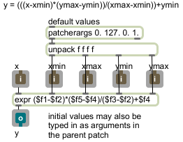
y = (((x-xmin)*(ymax-ymin))/(xmax-xmin))+ymin
This patch uses the expr object to implement that equation. In expr, the items such as $f1 and $f2 mean “the (floating point) number that has come in the first inlet”, “the (floating point) number that has come in the second inlet”, and so on. (Geeky technical note: We don’t need to use quite as many parentheses in the expr object as we did in the equation above, because the ordering of mathematical operations is implicit, due to the operator precedence that is standard in almost all programming languages.)
This patch has inlet objects and an outlet object so that it can be used as an object in another patch. You just save this patch with the name “lmap” somewhere in Max’s file search path, and you can then use it as a lmap object in any other patch. You establish the X and Y ranges by specifying their minimum and maximum (xmin, xmax, ymin, and ymax), then you send an x value in the left inlet to get the corresponding y value out the outlet. Thepatcherargs object supplies default initial values for xmin, xmax, ymin, and ymax in case no arguments are typed into the object when it’s created in the parent patch; however, if values are typed in for xmin, xmax, ymin, andymax (as in lmap 0. 1. -2. 2.), the patcherargs object inside lmap will send those values out instead of its default values.
Go ahead and download that patch and save it with the name “lmap”, as it will be used in the next example. In Max, patches that are saved with a one-word filename and used as objects in another patch are called “abstractions”. This lmap abstraction functions very much like the zmap object and scale object that already exist in Max, but I’ve provided lmap here so that you can see how one might implement the basic linear mapping function (in any language).
Linear mapping and linear interpolation
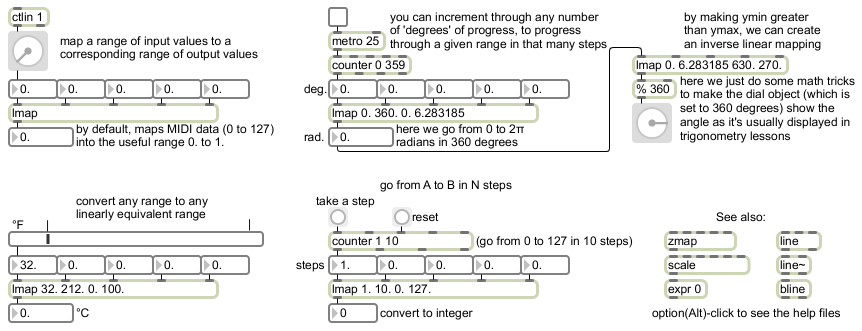
This patch shows examples of linear mapping and linear interpolation, using the lmap abstraction described above. One could substitute the built-in Max object scale in place of lmap with the same results.
As shown in the upper-left corner, with no arguments typed in lmap maps input values 0 to 127 (such as MIDI control data) into the range 0.0 to 1.0 (just as the scale object does by default). The output range 0.0 to 1.0 is useful for controlling the parameters of a lot of Jitter objects, and it’s also a range that can be re-mapped to any other range with simple scaling and/or offsetting (multiplication and/or addition).
Just below that is a mundane example of how linear mapping applies to common everyday conversion, such as converting temperatures from Fahrenheit to Celcius.
You can use linear mapping to step through any range in a specific number of N steps, just by setting an input range from 1 to N and providing input x values that count from 1 to N. This is demonstrated by the part of the patch labeled “go from A to B in N steps”. In effect, this is linear interpolation from A to B, since each step along the way will produce a corresponding intermediate value.
The part of the patch just above that demonstrates another case of the relationship between mapping and interpolation. The counter object counts cyclically in 360 steps from 0 to 359 (i.e., from 0 to almost 360), and we map the range 0 to 360 (the number of degrees in a circle) onto the output range 0 to 2π (the number of radians in a circle). Thus we’re able to go continually from 0 to (almost) 2π by degrees. (We then map that value with an inverse relationship in order to cause the dial to show the radial angle changing counterclockwise as it would be graphed in Cartesian trigonometry. Setting ymin to be greater than ymax causes such an opposite mapping.)
The Max objects line, line~, and bline offer three methods for linear interpolation within a single object.