Most of these basic programming constructs should be familiar to you, meaning you can read and interpret them and understand when and how to use them.

Students who do not have this background should take COGS 205A: Computational and Research Methods with MATLAB.

---

Matrices

Most MATLAB variables can be treated as matrices by default.

Constructing matrices

These are all fast ways to make matrices of one kind of another:

A = 3:9;                     % makes a 1x7 vector of consecutive integers 3..9
B = zeros(3);                % makes a 3x3 matrix of zeros
C = ones(3,2);               % makes a 3x2 matrix of ones
D = linspace(-pi,pi,pi/20);  % makes a vector starting at -pi ending at pi in steps of pi/20
E = rand(5);                 % makes a 5x5 matrix of uniform(0,1) random variates
F = randn(3,2,2);            % makes a 3x2x2 matrix of normal(0,1) random variates

The slow way of making matrices is using the [] operator:

G = [3 4 2; 1 2 0];          % makes a 2x3 matrix
H = [G; G];                  % makes a 4x3 matrix

Accessing

Individual elements or subsections of a matrix can be accessed directly:

A(3)        % third element of A is 5
B(2,2)      % second row, second column of B is 0
C(1,:)      % first row of C is [1 1]
D(end-1)    % second to last element of D is 19*pi/20
E(:,end)    % last column of E
F(:,:,2)    % second page of F

Updating

Any part of a matrix that can be accessed can be overwritten:

A(3) = 0;       % set third element of A to 0
C(1,:) = -1;    % set entire first row of C to -1
E(:,end) = [];  % remove last column from E

---

Basic operations

Not all MATLAB operations work the same way on matrices and scalar variables.

Arithmetic operations on scalars

1 + 2       % will return 3
2^4         % will return 16
5/2         % will return 2.5
1.4 * -2    % will return -2.8
4/0         % will return NaN

Arithmetic operations on matrices

Some operators are “element-wise” by default:

[1 2] + [-1 2]    % will return [0 4]
[1 2] - [-1 2]    % will return [2 0]

… but many operate differently on matrices than on scalars:

[1 2] * [-1 2]    % will give an error
[1 2] ^ [-1 2]    % will give an error
[1 2] / [-1 2]    % will not give an error but also not what you might expect!

Instead, use these element-wise operators:

[1 2] .* [-1 2]   % will return [-1 4]
[1 2] ./ [-1 2]   % will return [-1 1]
[1 2] .^ [-1 2]   % will return [1 4]

Scalar expansion

If you combine scalars and matrices in one expression, MATLAB can implicitly replace the scalar with a matrix of the appropriate size:

(1:4) - 1   % will return [0 1 2 3]

Logical operators

MATLAB knows a number of logical operators:

3 > 1                       % will return 1, for true
(1:4) <= 2                  % will return [1 1 0 0]
((1:3) < 3) & (4 < (4:6))   % will return [0 1 0]
(1:3) == 3 | (1:3) ~= 3     % will return [1 1 1]

Logical indexing

You can use logical expressions to index into a matrix or vector:

A = 1:5;
A(A ~= 3)    % will return [1 2 4 5]

---

Workspace management

MATLAB stores variables you make in its workspace.

who, whos      % list current variables
clear          % delete all variables
clear x y z    % delete only variables x, y, and z
save('nm')     % saves your current workspace as nm.mat
load('nm')     % loads the workspace from nm.mat  

Flow control

Flow control statements cause programs to skip some lines and repeat others.

If blocks

An if block only executes its contents if a condition is true.

variable  = 2;
condition = false;
if (condition)
    variable = 3;
end                  %  variable will be 2

If-else blocks

An if-else block executes one thing if a condition is true, and another thing if it is false.

variable  = 2;
condition = false;
if (condition)
    variable = 3;
else
    variable = 4;
end                  %  variable will be 4

For loops

A for loop repeats its contents once for each element of the index.

tracker = 0;
for ix = [1 1:3]
    tracker = tracker + ix;
end                  %  tracker will be 7

While loops

A while loop repeats its contents as long as a condition is true.

tracker = 0;
while tracker < 3
    tracker = tracker + 2;
end                  %  tracker will be 4

Try-catch blocks

A try-catch block executes one thing until there is an error, and then executes the other thing.

try
    B = [0 1];
    A = B*B; % will cause error
catch
    A = 0;
end                  %  A will be 0

---

Plotting

MATLAB has a wide variety of plotting tools.

Line plots

Use plot for basic line plots:

xax = linspace(-2, 2, 101);
yax = xax .^ 3;
plot(xax, yax)

Scatter plots

Use scatter to show the correlation between two dependent variables:

data = randn(100,2);
scatter(data(:,1), data(:,2))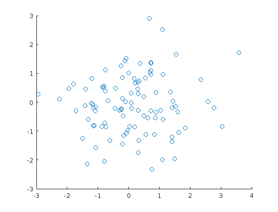

Bar charts

Use bar for basic line plots:

xax = 1:4;
yax = [5 9 1 2];
bar(xax, yax)