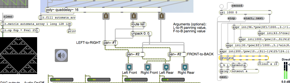
pinger: a beeping test sound.
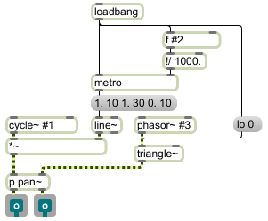
This patch is designed to be used as an abstraction (subpatch) in the next example. In order for the next example to work, you should download this example and save it with the filename “pinger.maxpat” somewhere in the Max file search path.
Its purpose is just to generate a recognizable sound. It emits very short sinusoidal beeps of a specified frequency, at a rate of a specified number of beeps per second, panning back and forth from left to right a specified number of times per second. These three parameters — tone frequency, note rate, and panning rate — are specified as arguments 1, 2, and 3 in the parent patch.
Because this abstraction was designed just to be used as a test tone in a particular example, it just uses the simple #1, #2, and #3 arguments as a way of providing the parameter values (as unchangeable constants typed in the parent patch). To make a more versatile program, one could also provide inlets to receive variable values, and could use patcherargs to provide useful default initial values. Compare, for example, the lmap abstraction.
Mixing multiple audio processes
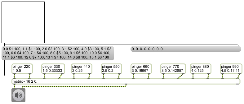
For this example to work correctly you will need to first download the pinger abstraction above and save it with the filename “pinger.maxpat” somewhere in the Max file search path.
This example shows the use of the matrix~ object to mix together different sounds. Think of matrix~ as an audio mixer/router (a kind of combination of mixer and patch bay). The first two arguments specify the number of inlets and outlets, and the third argument specifies the default gain factor for each inlet-outlet connection.
Inlets and outlets of matrix~ are numbered starting from 0. So, in this example there are 16 inlets (numbered 0 to 15) and 2 outlets (numbered 0 to 1). (There’s always an extra outlet on the right, from which informational messages are sometimes sent.)
Messages to the left inlet of matrix~ generally take the form of a four-item list to specify an inlet, an outlet to be connected that inlet, a gain factor (multiplier) for sounds that will flow from that inlet to that outlet, and a ramp time to transition smoothly to that gain factor (to avoid clicks). You can send as many such messages as you’d like, to specify as many connections as you want.
In this example we have connected eight stereo pinger objects to the 16 inlets of matrix~, and we will mix them all together for a single stereo output. The pinger objects are just stand-ins for what could potentially be any eight different audio processes you might want to mix together. The arguments to pinger specify frequency of the beep tone, the number of notes per second, and the rate of panning. For example, the first pinger plays a 220 Hz tone 1 time per second (i.e., at a rate of 1 Hz), panning left to right once every two seconds (i.e. at a rate of 0.5 Hz). The next pinger plays a 330 Hz tone at a rate of 1.5 notes per second (i.e. once every 666.6667 milliseconds), panning left to right once every three seconds (i.e., at a rate of 0.33333 Hz), and so on. The result is 8 tones (harmonics 2 through 9 of the fundamental frequency of 110 Hz) at 8 different harmonically-related rhythmic rates, panning back and forth at 8 different harmonically-related rhythmic rates.
With matrix~ you can mix these eight tones in any proportion you want, but how can you easily control all eight amplitudes at once? If you had a MIDI fader box, you could map the eight control values from the faders to the gain factors of the various connections. In the absence of such a fader box, we use the multislider object, set to have 8 sliders, that sends out a list of eight values from 0. to 1. corresponding to the vertical position of each slider as drawn with the mouse. So, by clicking and/or dragging with the mouse on the multislider you can set eight level values for use by matrix~. That list of eight values is sent to the right inlet of the right message box so we can see the values, and it’s also sent to the left inlet of the left message box where the values are used in sixteen different connection messages to matrix~.
Take a moment to examine and understand those messages. The first message says “connect the first inlet [inlet 0] to the first outlet [outlet 0] multiplied by a gain factor [the value of the first slider] with a transition time of 100 milliseconds, and so on. Each pair of messages controls a pair of inlets corresponding to one of the pingers, and sets the gain with which that pinger will go to the output.
Turn on audio audio by clicking on the ezdac~, then try out the patch by moving the sliders in the multislider. Note that when you add together eight different audio processes, each playing at full volume, you need to be careful about the sum of all your gain factors. A more elaborate patch would, at the least, provide a volume control for the final summed signal. Even more desirably, perhaps, the final volume control could be constantly controlled automatically, proportionally to the sum of the slider values, to prevent clipping of the output signal.