The phasor~ object

Image

The phasor~ object is one of the most valuable MSP signals to use as a control signal. (You wouldn’t generally want to listen to it directly as audio because it’s an ideal sawtooth wave and has energy at so many harmonics that it can easily create aliasing. If you want a sawtooth wave sound, it’s better to use the saw~ object, which limits its harmonics so as not to exceed the Nyquist frequency.) The phasor~ outputs a signal that ramps cyclically from 0 to 1. It’s actually more correct to say that phasor~ ramps from 0 to almost 1, because it will never actually output the value 1; it will instead output 0 because the end of a ramp is the same moment as the beginning of the next ramp. Because phasor~ is constantly moving and interpolating between 0 and 1, it’s usually best not to rely on detecting any specific value in its output signal, but just to know that it’s always increasing linearly from 0 toward 1.

Random access of a sound sample

Image


The fact that groove~ can leap to any point in the buffer~ makes it a suitable object for certain kinds of algorithmic fragmented sound playback. In this example it periodically plays a small chunk of sound chosen at random (and with a randomly chosen rate of playback).

The info~ object reports the length of the sound that has been read into the buffer~, and that number is used to set the maximum value for the random object that will be used to choose time locations. When the metro is turned on, its bangs trigger three things: an amplitude envelope, a starting point in ms, and a playback rate. The starting point is some randomly chosen millisecond time in the buffer~. The rate is calculated by choosing a random number from 0 to 200, offsetting it and scaling it so that it is in the range -1 to 1, and using that number as the exponent for a power of 2. That’s converted into a signal by the sig~ object to control the rate of groove~. (2 to the -1 power is 0.5, 2 to the 0 power is 1, and 2 to the 1 power is 2, so the rate will always be some value distributed exponentially between 0.5 and 2.)

The amplitude envelope is important to prevent clicks when groove~ leaps to a new location in the buffer~. The line~ object creates a trapezoidal envelope that is the same duration as the chunk of sound being played. It ramps up to 1 in 10 milliseconds, stays at 1 for some amount of time (the length of the note minus the time needed for the attack and release portions), and ramps back to 0 in 10 ms. Notice that whenever the interval of the metro is changed, that interval minus 20 is stored and is used as the sustain time for subsequent notes. This pretty effectively creates a trapezoidal “window” that fades the sound down to 0 just before a new start time is chosen, then fades it back up to 1 at the time the new note is played.

MSP calculates audio signals several samples at a time, in order to ensure that it always has enough audio to play without ever running out (which would cause clicks). The number of samples it calculates at a time is determined by the signal vector size, which can be set in the Audio Status window. If the sample rate is 44100 Hz, and the signal vector size is 64, this means that audio is computed in chunks of 1.45 ms at a time; a larger signal vector size such as 512 would mean that audio is computed in chunks of 11.61 ms at a time. For this reason, the millisecond scheduler of Max messages might not be in perfect synchrony with the MSP calculation interval based on the signal vector size. This causes the possibility that we will get clicks even if we are trying to make Max messages occur only at moments when the signal is at 0. For that reason, you need to be very careful to synchronize those events carefully. One thing that can help is to synchronize the Max scheduler to send messages only at the same time as the beginning of a signal vector calculation. You can do that by setting the Scheduler in Overdrive and Scheduler in Audio Interrupt options both On in the Audio Status window. Another useful technique (although not so appropriate with groove~, which can only have its starting points triggered by Max messages) is to cause everything in your MSP computations to be triggered by other signals instead of by Max messages.

Playing a sample with groove~

Image


The groove~ object plays sound from a buffer~, using two important pieces of information: a rate provided as a MSP signal and a starting point provided as a float or int message. For normal playback, the rate should be a signal with a constant value of 1. (The sig~ object is a good way to get a constant signal value.) A rate of 2 will play at double speed, a rate of 0.5 will play at half speed, and so on. Negative rate values will play backward. The starting point is stated in milliseconds from the beginning of the buffer~. In the example patch, read some sound into the buffer~ objects, turn up the gain~, send a starting point number to groove~’s left inlet from the number box, and set the sig~ value to 1. The sound will play till the end of the buffer~ is reached or until the rate is set to 0 (or until a new starting point is sent in the left inlet.)

You can use a ‘set’ message to groove~ to cause it to access a different buffer~. All its other settings will stay the same, but it will simply look at the new buffer~ for its sample data. You can test this by clicking on the ‘set soundA’ and ‘set soundB’ message boxes.

One of the important features of groove~ is that it can be set to loop repeatedly through a certain segment of the buffer~. You set groove~’s loop start and end times (in ms) with numbers in the second and third inlets. By default, looping is turned off in groove~, but if you send it a ‘loop 1’ message it will play till the loop end point, then leap back to the loop start point and continue playing. When looping is turned off, the loop end point will be ignored and groove~ will play till the end of the buffer~. To loop the entire buffer~, set the loop start and end times to 0. (An end time of 0 is a code to groove~ meaning “the end of the buffer~”.)

You can also cause groove~ to start playing from the loop start time with the ‘startloop’ message. This works even when looping is turned off, but the loop end point will be ignored if looping is turned off. (Note that ‘startloop’ does not mean “turn looping on”; it means “start playing from whatever time is set as the loop start time”.)

Whenever groove~ leaps to a new point in the buffer~ — either because of a float or int message in its left inlet, or with a ‘startloop’ message, or by reaching its loop end time and leaping back to the loop start time — there is a potential to cause a click because of a sudden discontinuity in the sound.

DJ-like sample scrubbing

Image


Although playback is normally achieved by progressing linearly through a stored sound, other ways of traversing the sound can give interesting results. Moving quickly back and forth in the sound is analogous to the type of “scrubbing” achieved by rocking the reels of a tape recorder back and forth by hand, or by “scratching” an LP back and forth by hand. In this example, we use a cycle~ object to simulate this sort of scrubbing. The output of cycle~ is normally in the range -1 to 1, so if we want its output to be used as the playback position in milliseconds, we need to scale its output with a *~ object and offset it with a +~; the multiplication will determine the depth (range) of the scrubbing, and the addition will determine the center time around which the scrubbing takes place. Initially the patch is set to scrub the entire range of the buffer~ in a time span (period) of 40 seconds. You can get different results by changing, in particular, the rate and depth values. For example, with a depth of about 250 milliseconds and a rate of about 3 Hz, you can get a sound that’s much more like tape reel scrubbing or LP scratching.

Sample playback driven by a signal

Image


The play~ object can be controlled by any MSP signal in its inlet. The value of the signal controls the location in the buffer~, in milliseconds. Normal playback can be achieved in this way by using a linear signal, such as from a line~ object, that traverses a given time span in the expected amount of time. By making a signal that goes linearly from a starttime to a stoptime in a certain amount of time, line~ can be used to get the same sorts of playback as with the ‘start’ message with three arguments demonstrated in the previous example.

In this patch you can see how the line~ object is commanded to leap to a particular value, then proceed to a new value linearly in a certain amount of time. The existence of a comma in a message box divides the message into two separate messages, sent out in succession as quickly as possible. So a message such as ‘0, 2000 2000’ sends out the int message ‘0’ followed immediately by the list message ‘2000 2000’. The int causes line~ to go to the value immediately, and the list causes line~ to use the number pair(s) as destination and ramptime. So the first message says, “Go to 0 immediately, then proceed toward 2000 in 2000 milliseconds.” This will result in normal forward playback. Going from 2000 to 0 in 2000 milliseconds causes backward playback at normal speed. Going from 0 to 420 in 525 milliseconds causes the playback to be at 4/5 normal speed, which also causes downward transposition by a major third.

Playing a sample from RAM

Image

You can use the play~ object to play the contents of a buffer~, simply by sending it a ‘start’ message. By default it starts from the beginning of the buffer~. You can specify a different starting time, in milliseconds, as an argument to the ‘start’ message, or you can specify both a starting time and a stopping time (in ms) as two arguments to the ‘start’ message. In the patch, you can see two examples of the use of starttime and stoptime arguments. The message ‘start 0 420’ reads from time 0 to time 420 ms, then stops. You can cause reverse playback just by specifying a stop time that’s less than the start time; the message ‘start 2000 420’ starts at time 2000 ms and plays backward to time 420 ms and stops. In all of these cases — start with no arguments, start with one argument, or start with two arguments — play~ plays at normal speed. If you include a third argument in the ‘start’ message, that’s the amount of time you want play~ to take to get to its destination; in that way, you can cause play~ to play at a different rate, just by specifying an amount of time that’s not the same as the absolute difference between the starttime and stoptime arguments. For example, the message ‘start 1000 2000 1200’ means “play from time 1000 ms to time 2000 ms in 1200 ms.” Since that will cause the playback to take 6/5 as long as normal playback, the rate of playback will be 5/6 of normal, and thus will sound a minor third lower than normal. (The ratio between the 5th and 6th partials of the harmonic series is a pitch interval of a minor third.) The message ‘start 2000 1000 4000’ will read backward from 2000 ms to 1000 ms in 4000 ms, thus playing backward at 1/4 the original rate, causing extreme slowing and a pitch transposition of two octaves down.

The info~ object, when it receives a bang in its inlet, provides information about the contents of a buffer~ object. Since the buffer~ object sends a bang out its right outlet when it has finished a ‘read’ or ‘replace’ operation, we can use that bang to get information about the sound that has just been loaded in. In this example, we see the length of the buffer, in milliseconds. You can use that information in other parts of your patch.

Simple wavetable synthesis

Image


One of the earliest methods of digital sound synthesis was a digital version of the electronic oscillator, which was the most common sound generator in analog synthesizers. The method used was simply to read repeatedly, at the established sample rate, through a stored array of samples that represent one cycle of the desired sound wave. By changing the step size with which one increments through the stored wavetable, one can alter the number of cycles one completes per second, which will determine the perceived fundamental frequency of the resulting tone. For example, if the sample rate (R) is 44100 and the length of the wavetable (L) is 1000 samples, and our increment step size (I) is an expected normal step of 1, the resulting frequency (F) will be F=IR/L which is 44.1 Hz. If we wanted to get a different value for F, while keeping R and L constant, we can just change I, the step size. For example, if we use an increment of 2, leaping over every other sample, we’d get through the table 88.2 times in one second. Thus, by changing I, we can get a cyclic tone of any frequency, and it will have the shape of the waveform stored in the wavetable. (When I is a non-integer number, it will result in trying to read samples at non-existent fractional indices in the wavetable. In those cases, some form of interpolation between adjacent samples is used to get the output value.)

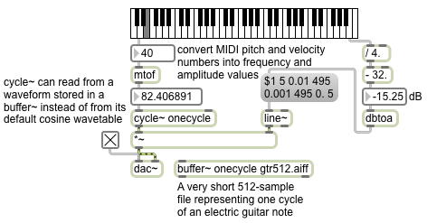
When a cycle~ object refers to a buffer~ by name, it uses the first 512 samples of that buffer~ as its waveform, instead of using its default cosine waveform. In this example, the buffer~ is loaded with a 512-sample file that is actually a single cycle of an electric guitar note. (The file is in the Applications/Max6/patches/docs/tutorial-patchers/msp-tut/ folder of your hard drive, which is probably already included in your file search path, so it should load in automatically.) The frequency value supplied in the left inlet of cycle~ determines the increment I value that cycle~ will use to read through that wavetable. So for this example, we use a MIDI-type pitch number from the left outlet of the kslider and convert it to frequency with the mtof object (which uses a formula such as [expr 440.*pow(2.\,($f1-69.)/12.)] to convert from MIDI pitch number to frequency in Hz). We also use the MIDI-type “velocity” value from the kslider to determine the amplitude of the sound. The velocity value is scaled and offset to give a decibel range between -32 dB and 0 dB; that is used as the peak (attack) amplitude in an amplitude envelope sent to the line~ object to control the amplitude of the cycle~. The amplitude envelope goes to the peak amplitude in 5 ms, then falls to 0.01 (-40 dB) in 495 ms, then falls further to 0.001 (-60 dB) in 495 more ms, and finally goes to 0. (-infinity dB) in 5 ms; so the whole envelope shapes a 1-second note.

Notice that when you play high notes on the keyboard, the tone becomes inharmonic. That’s because the stored waveform in the buffer~ is so jagged and creates so many harmonics of the fundamental pitch. When the fundamental is high (in the top octave of this keyboard the fundamental frequencies are all above 1000 Hz) upper harmonics of the tone get folded back due to aliasing, resulting in pitches that don’t belong to the harmonic series of the fundamental.

Getting a sound sample from RAM

Image


The buffer~ object holds audio data in RAM as an array of 32-bit floating point numbers (floats). The fact that the sound is loaded into RAM, rather than read continuously off the hard drive as the sfplay~ object does, means that it can be accessed quickly and in various ways, for diverse audio effects (including normal playback).

Every buffer~ must have a unique name as its first argument; other objects can access the contents of the buffer~ just by referring to that name. The next (optional) arguments are the size of the buffer (stated in terms of the number of milliseconds of sound to be held there) and the number of channels (1 for mono, 2 for stereo). If those optional arguments are present, they will be used to limit the amount of sound that can be stored in that buffer~ when you load sound into the buffer~ from a file with the ‘read’ message. If those arguments are absent, when you load in a sound from a file with the ‘read’ message the buffer~ will be resized to to hold the entire file. The ‘replace’ message is like ‘read’ except that it will always resize the buffer~ regardless of the arguments.

The most basic way to use a buffer is simply to access each individual sample by incrementing through the array indices at the sample rate. To do that, the best objects to use are count~, which puts out a signal that increments by one for each sample, and index~, which refers to the buffer~’s contents by the sample index received from count~ and sends that out its outlet. This is good for basic playback with no speed change, or for when you want to access a particular sample within the buffer~.

When count~ receives a ‘bang’, it begins outputting an incrementing signal, starting from 0 by default. You can cause it to start counting from some other starting sample number by sending a number in its left inlet. (You can also cause it to count in a loop by giving it both a starting and ending number. It will count from the starting number up to one less than the ending number, then will loop back to the starting number.)

Constant power panning using table lookup

Image


In the previous example we used the square root of the desired intensity for each speaker to calculate the amplitude of each speaker. However, square root calculations are somewhat computationally intensive, and it would be nice if we could somehow avoid having to perform two such calculations for every single audio sample. As it happens, the sum of the squares of sine and cosine functions also equals 1. So, instead of using the square roots of numbers from 0 to 1 (and their complements) to calculate the amplitude for each speaker, we can just look up the sine and cosine as an angle goes from 0 to π/2 (the first quarter of the cosine and sine functions).

In this patch, therefore, we scale the panning value down to a range from 0 to 0.25 and we use that as the phase offset in a 0 Hz cycle~ object. As the panning value moves from 0 to 1, the left speaker’s amplitude is looked up in the first quarter of a cosine function and the right speaker’s amplitude is looked up in the first quarter of a sine function (by adding an additional 0.75 to the scaled phase offset). The resulting effect is just the same as if we performed the square root calculation, but is less computationally expensive.

In most cases this is the preferred method of constant-power intensity panning between stereo speakers. It’s so generally useful that it’s worthwhile to implement it and save it as an abstraction, for use as a subpatch in any MSP program for which stereo panning is required. An abstraction version of this method is demonstrated in Example 43 from the 2009 class.

Constant power panning using square root of intensity

Image


The intensity of sound is proportional to the square of its amplitude. So if we want to have a linear change in intensity as we go from 0 to 1 or 1 to 0, we need to use the square root of that linear change to calculate the amplitude. This example patch is exactly like the previous example, except that we consider the linearly changing signal from line~ to be the intensity rather than the amplitude, and we take the square root of that value to obtain the actual amplitude for each speaker. By this method, when the sound is panned in the center between the two speakers, instead of the amplitude of each speaker being 0.5, it will be the square root of 0.5, which is 0.707 (which is an increase of 3 dB compared to 0.5). This compensates for, and effectively eliminates, the undesirable ‘hole-in-the-middle’ effect discussed in the previous example.