Transport-controlled phasor~

Image


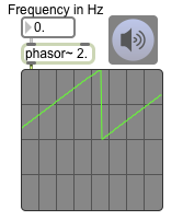
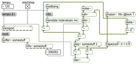
A phasor~ object, like other MSP objects such as cycle~ that use a rate for their timing, can have its repetition rate specified as a transport-related tempo-relative time value (note values, ticks, etc.). So if you want a phasor~ to work at a rate that is related to the transport’s tempo, you can type in a tempo-relative time as an argument to specify its period of repetition instead of typing in a frequency. The existence of that time syntax argument will tell the object to use the transport’s tempo as its basis of timing. MSP objects that are using transport-based timing will work — and will respond to changes in the transport’s tempo — even when the transport is not turned on. By setting the object’s ‘lock’ attribute to 1, you can cause the object to sync precisely to the quantized note value of the moving transport. When the lock attribute is on, the object will only work when the transport is on.

In this example we have a phasor~ with a typed-in argument of 16n and a lock attribute setting of 1. This means that it will only move forward when the transport is running, and its period of repetition will be synchronized with the 16th notes of the transport.

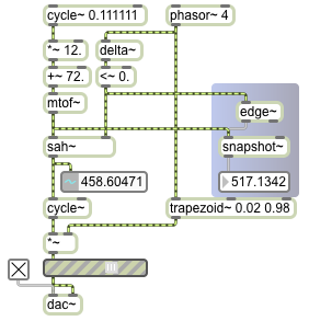
Read some sound into the buffer~. This will cause the length of the sound file to go to the right inlet of the *~ object. The noise~ object generates random sample values in the range -1 to 1. We use the sample-and-hold trick that was explained in Example 25 to get individual random numbers at a time that’s perfectly synchronized with the start of each phasor~ cycle, we take the absolute value of that (to force the number to be positive) scale it to be a useful time value within the buffer~, and use that as a starting point for play~ each time the phasor~ starts a new ramp. By translating the 16th-note note value into milliseconds, we can scale the phasor~ ramp to traverse one 16th note’s worth of time in the play~ object, offset by the starting point we got from sah~. The same phasor~ is used to make a trapezoidal amplitude envelope for each 16-note chunk of audio we play. The result is randomly-chosen 16th-note soundbites played continuously and in synchrony with the transport (and click-free) from the buffer~.

Triggering events with each cycle of a phasor~

Image

How do we detect, with sample-accurate precision, the precise moment when phasor~ begins a new cycle from 0 to 1? We need to detect the sample on which it leaps from 1 back to 0. However, because phasor~ is constantly interpolating between 0 and 1, it might not leap down to exactly 0. So we can’t just use a ==~ object to see when its value is 0. Its exact value is relatively unknowable with any great precision; all we know is that it’s always increasing…except at the one instant when it leaps back down to (approximately) 0 and begins again. However, that instant is so remarkable that there is a way to detect it, with the help of an object called delta~. A delta~ object sends out a signal in which each sample reports the change in its input relative to the previous sample. So, if we send a phasor~ into a delta~, delta~ will always report a positive increase (or 0 if the phasor~ is completely stopped), except for when the phasor~ leaps downward. That’s the one sample on which delta~ will report a negative value. So we can use a <~ 0 object to detect the sample on which that occurs. The <~ 0 object will always output a signal of 0 (false) except for that one sample when it will report a 1 (true).

The sah~ object implements a “sample-and-hold” mechanism. When a particular threshold is surpassed in the signal in its right inlet, it will sample the value of the signal in its left inlet and will hold that as a constant output signal value until the next time the threshold is surpassed in the right inlet. By default its threshold is 0, so every time the <0~ object sends out a 1 preceded by a 0 it will cause sah~ to sample its left input. We use that fact to sample the slowly moving sinusoidal control value coming from cycle~ via mtof~. The cycle~ is moving slowing with a period of 9 seconds, and it’s varying + or – 12 semitones from a central pitch of 72 (C above middle C); that signal value is converted to frequency by the mtof~ (MIDI to frequency) object and that is sampled and held 4 times per second by the sah~ which is triggered by the phasor~. That frequency value from sah~ — which is constant for each 1/4 second until it is changed by sah~ — is used by cycle~ as its frequency value for its notes.

The individual notes are shaped by a trapezoidal amplitude envelope. The envelope is almost rectangular, but it has a very quick ramp up and down during the first and last 2% of each note (5 ms in this case). Because the change in frequency of the cycle~ that we’re listening to is triggered by the beginning of each cycle~ of the phasor~, it’s perfectly synchronized with the trapezoidal amplitude envelope.

If you want to use the beginning of a phasor~ ramp to trigger events in other parts of a Max patch, you can use an edge~ object to detect the 1 values coming from the <~ 0 object. The edge~ will send out a bang when a 0-to-1 or 1-to-0 transition occurs in a signal vector. But it can only do so with as much precision as the Max scheduler provides, which is not sample-accurate. So in this patch we use edge~ to detect the 0-to-1 transitions, then we use that bang to trigger a report of the current frequency value with a snapshot~ object. Note that not only will the edge~ object not send a bang with sample-rate precision, snapshot~ will only report the value at the beginning of the signal vector when (or immediately after) it receives the bang. So these translations between the sample-accurate-but-vector-based timing of MSP and the millisecond (or vector-based) timing of the Max scheduler show the slight difference between the true sample-accurate timing of the phasor~ and the close approximation that we can achieve with edge~. When you stop the audio (by turning off the dac~), you will probably notice a slight difference between the actual frequency being reported by the number~ object and the frequency reported by snapshot~ at the beginning of the vector when it was triggered by edge~. In many cases this difference is negligible, but in some cases it can lead to clicks when sudden changes are made in an audio signal that is not at 0 amplitude.

Repeatedly reading a function with phasor~

Image


The real value of phasor~ is that it provides a very accurate way to read through (or mathematically calculate) some nonlinear shape to use as a control signal (or even as an audio signal). Among other things, it might be used to create a “window” shape that can serve as an amplitude envelope for a sound. This patch demonstrates five different ways to create window or waveform shapes with phasor~. We’ll discuss them (in good Max fashion) from right to left.

The trapezoid~ object expects a signal that progresses from 0 to 1. It has two arguments (or values it can receive): one to say at what point its upward ramp should end, and the other to say at what point its downward ramp should begin. So in this example, as the phasor~ signal goes from 0 to 1, the trapezoid~ object will ramp upward and arrive at 1 just as phasor~ gets to 0.25 (the first argument of trapezoid~), then trapezoid~ will stay at 1 till phasor~ gets to 0.75 (the second argument of trapezoid~) at which point trapezoid~ will begin to ramp back down to 0 and will arrive there just as phasor~ completes its cycle. This can be useful for tapering the ends of some other signal (such as notes or loops played by a groove~ object) to avoid clicks.

The triangle~ object similarly makes a simple shape when driven by a signal between 0 and 1. The first argument of triangle~ specifies where in the phasor~’s 0-to-1 range the highpoint of the triangle should occur, and the lo and hi attributes specify the minimum and maximum output values.

The output of phasor~ can be used to control the phase offset of a cycle~ object (in cycle~’s right inlet). If the cycle~’s frequency is 0, the signal from phasor~ will specify the exact location (on a scale from 0 to 1) in the wavetable that cycle~ will send out. Since cycle~ uses a cosine wavetable by default, scanning through the entire wavetable (0 to 1) in this way would cause cycle~ to output a cosine wave. However, in this example we scale and offset the phasor~ signal so that it goes cyclically from -0.25 to 0.25, thus cycling through the first half of a sine wave. This creates a window shape that’s commonly called a cosine window, which is also useful as an amplitude envelope, particularly for short notes.

Because the cycle~ object can use a buffer~ as a wavetable (see Example 16 above), we can fill a buffer~ with 512 samples of any shape we want, and then read through that function with cycle~. The buffer~ object even has a few messages for doing just that. In this patch we have created a buffer~ called “useasawindow”, we set its size to 512 samples, we fill it with all values of 1, and then we impose a “hanning” (or “Hann”) window on it. (A hanning window is really just cosine waveform that has been scaled and offset.)

The wave~ object can also access samples in a buffer~ in a fashion similar to a cycle~ (with frequency 0) driven by a phasor~. A difference with wave~ is that it can use any portion of a buffer~ as its wavetable. You specify the start and end points (in ms) of the portion of the buffer that you want to use, and wave~ will use that as its wavetable to read when it is driven by a signal from 0 to 1. In this patch we use a small portion (about one cycle) of a cello note. When phasor~ is at a very low subaudio frequency (such as 1 Hz.) you can see the waveform pretty clearly in the scope~. To hear it, raise the phasor~ to an audio frequency (and turn up the gain~). As you change the range of the buffer~ that is being accessed by wave~, the timbre of the tone will change (because the resulting waveform is changing), but the fundamental frequency of the wave is still largely determined by the rate of the phasor~.

Using phasor~ directly as a control signal

Image


If you need a linear signal that repeats at a specific rate, phasor~ can be scaled and offset to provide a repeating line from one signal value to another. In this example, we use phasor~ to directly control both frequency and amplitude of an oscillator.

Since phasor~ ramps from 0 to (almost) 1, it would normally create a crescendo in amplitude, and indeed it can be useful for that purpose over long periods of time as a control signal for other control signals. A more normal amplitude envelope for a single note, however, goes quickly to a peak amplitude and then gradually decreases to 0 over the course of the note. So in this patch we multiply the phasor~ signal by -0.5, which causes it to ramp from 0 to -0.5, and then we add 0.5 to that so that it is now ramping from 0.5 to 0. (Notice that the leap up from 0 to 0.5 is instantaneous, though, causing a click in this case. A more sophisticated program might do something to smooth that transition.) We use a similar scaling and offsetting procedure for the control of frequency of the cycle~. We multiply the phasor~’s output by 500 then add 500 to that so that the result is a ramp that goes from 500 to 1000 (a number that we use as Hz in the cycle~). You can experiment with other rate settings for the phasor~ and other frequency ranges for the cycle~.

The phasor~ object

Image

The phasor~ object is one of the most valuable MSP signals to use as a control signal. (You wouldn’t generally want to listen to it directly as audio because it’s an ideal sawtooth wave and has energy at so many harmonics that it can easily create aliasing. If you want a sawtooth wave sound, it’s better to use the saw~ object, which limits its harmonics so as not to exceed the Nyquist frequency.) The phasor~ outputs a signal that ramps cyclically from 0 to 1. It’s actually more correct to say that phasor~ ramps from 0 to almost 1, because it will never actually output the value 1; it will instead output 0 because the end of a ramp is the same moment as the beginning of the next ramp. Because phasor~ is constantly moving and interpolating between 0 and 1, it’s usually best not to rely on detecting any specific value in its output signal, but just to know that it’s always increasing linearly from 0 toward 1.