Tag Archives: random
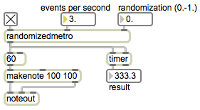
Demonstration of the randomizedmetro subpatch
Image
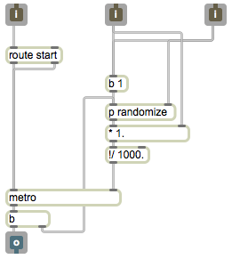
Metronome with random perturbations of tempo
Image
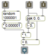
Generate random numbers within a specified range
Image
Random note choices
Image
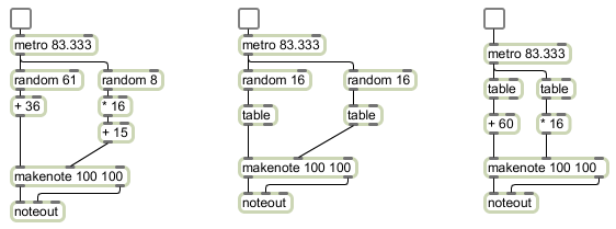
The left part of this example shows the use of the random object to make arbitrary note choices. Every time random receives a bang in its inlet, it sends out a randomly chosen number from 0 to one less than its argument. In this case it chooses one of 61 possible key numbers, sending out a number from 0 to 60. We then use a + object to offset that value by 36 semitones, transposing up three octaves to the range 36 to 96 — cello low C to flute high C. Similarly, we choose one of 8 possible velocities for each note. The random object sends out a number from 0 to 7, which we scale by a factor of 16 and offset by 15, thus yielding 8 possible velocities from 15 to 127. These choices by the random objects are made completely arbitrarily (well, actually by a pseudo-random process that’s too complex for us to detect any pattern), so the music sounds incomprehensible and aimless.
One can make random decisions with a little bit more musical “intelligence” by providing the computer with a little bit of musically biased information. Instead of choosing randomly from all possible notes of the keyboard, one can fill a table with a small number of desirable notes, and then choose randomly from among those. In the middle example, we have filled lookup tables with 16 possible velocity values and 16 possible pitches. Each time we want to play a note, we choose randomly from those tables. The velocities are mostly mezzo-forte, with only one possible forte value and one fortissimo value. Thus, we would expect that most notes would be mezzo-forte, with random accents occurring unpredictably on (on average!) one out of every eight notes. The pitches almost all belong to a Cm7 chord, with the exception of a single D and a single A in the upper register. So, statistically we would expect to hear a Cm7 sonority with an occasional 9th or 13th. There’s no strong sense of melodic organization, because each note choice is made by random with no regard for any previous or future choices, but the limited, biased set of possibilities lends more musical coherence to the results.
In a completely different usage of the table object, you can use table as a probability distribution table, by sending it bang messages instead of index numbers. When table receives a bang, it treats its stored values as relativeprobabilities, and sends out a chosen index number (not the value stored at that index) with a likelihood that corresponds to the stored probability at that index. Double-click on the table objects in the right part of the patch to see the probabilities that are stored there. In the velocity table, you can see that there is a relatively high probability of sending out index numbers 4 or 5, and a much lesser likelihood of sending out index numbers 1 or 7. These output numbers then get multiplied by 16 to make a MIDI velocity value. Thus we would expect to hear mostly mezzo-forte notes (velocities 64 or 80) and only occasional soft or loud notes (velocities 16 or 112). In the pitch table, you can see that the index numbers with the highest probabilities are 0, 4, 7, and 11 respectively, with a very low likelihood of 2, 9, or 12. These values have 60 added them to transposed them to the middle octave of the keyboard. So we would expect to hear a Cmaj7 chord with only a very occasional D or A.
To learn more about the use of table to get weighted distributions of probabilities, read the blog article on “Probability distribution”.
Some objects for generating numbers
Image
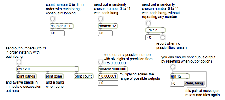
This patch shows four objects that are useful for generating numbers, each with a different behavior. The arguments to these objects determine how many different possible numbers the object will generate, and the range of those numbers. The range can be changed, though, by ‘scaling’ (multiplying) them and/or by ‘offsetting’ (adding something to) them.
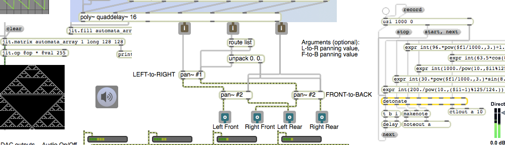
Random access of a sound sample
Image
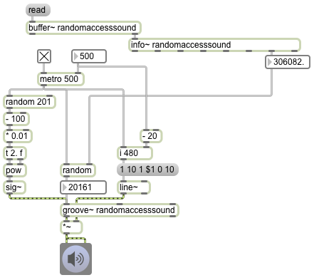
The fact that groove~ can leap to any point in the buffer~ makes it a suitable object for certain kinds of algorithmic fragmented sound playback. In this example it periodically plays a small chunk of sound chosen at random (and with a randomly chosen rate of playback).
The info~ object reports the length of the sound that has been read into the buffer~, and that number is used to set the maximum value for the random object that will be used to choose time locations. When the metro is turned on, its bangs trigger three things: an amplitude envelope, a starting point in ms, and a playback rate. The starting point is some randomly chosen millisecond time in the buffer~. The rate is calculated by choosing a random number from 0 to 200, offsetting it and scaling it so that it is in the range -1 to 1, and using that number as the exponent for a power of 2. That’s converted into a signal by the sig~ object to control the rate of groove~. (2 to the -1 power is 0.5, 2 to the 0 power is 1, and 2 to the 1 power is 2, so the rate will always be some value distributed exponentially between 0.5 and 2.)
The amplitude envelope is important to prevent clicks when groove~ leaps to a new location in the buffer~. The line~ object creates a trapezoidal envelope that is the same duration as the chunk of sound being played. It ramps up to 1 in 10 milliseconds, stays at 1 for some amount of time (the length of the note minus the time needed for the attack and release portions), and ramps back to 0 in 10 ms. Notice that whenever the interval of the metro is changed, that interval minus 20 is stored and is used as the sustain time for subsequent notes. This pretty effectively creates a trapezoidal “window” that fades the sound down to 0 just before a new start time is chosen, then fades it back up to 1 at the time the new note is played.
MSP calculates audio signals several samples at a time, in order to ensure that it always has enough audio to play without ever running out (which would cause clicks). The number of samples it calculates at a time is determined by the signal vector size, which can be set in the Audio Status window. If the sample rate is 44100 Hz, and the signal vector size is 64, this means that audio is computed in chunks of 1.45 ms at a time; a larger signal vector size such as 512 would mean that audio is computed in chunks of 11.61 ms at a time. For this reason, the millisecond scheduler of Max messages might not be in perfect synchrony with the MSP calculation interval based on the signal vector size. This causes the possibility that we will get clicks even if we are trying to make Max messages occur only at moments when the signal is at 0. For that reason, you need to be very careful to synchronize those events carefully. One thing that can help is to synchronize the Max scheduler to send messages only at the same time as the beginning of a signal vector calculation. You can do that by setting the Scheduler in Overdrive and Scheduler in Audio Interrupt options both On in the Audio Status window. Another useful technique (although not so appropriate with groove~, which can only have its starting points triggered by Max messages) is to cause everything in your MSP computations to be triggered by other signals instead of by Max messages.