Many interesting audio effects are achieved by combining a sound with a delayed (and possibly altered) version of itself. To delay a sound, one needs to store it for a certain amount of time till (a delayed copy of) it is needed. That storage has to be constantly ongoing when we’re dealing with realtime audio processing, yet we usually also want to dispose of the delayed audio data once it’s no longer needed. Realtime delay of audio is therefore most often achieved by storing the sound in what’s commonly called a ring buffer or a circular buffer.

In MSP a circular buffer is implemented in the delay~ object, and also in the pair of objects called tapin~ and tapout~. Here are some examples from a previous class.
Simple delay of audio signal
Delay with tempo-relative timing
Simple flanging
Delay with feedback

There are some MSP Tutorials that deal with delayed sound. [The links below are to the web version of the documentation, but you’ll probably prefer to use the Reference documentation within Max so that you can try out the tutorial patches while you read about them.]
Delay Lines
Delay Lines with Feedback
Flanging
Chorus
Comb Filter

And here are some more examples from a past class.
Change of delay time may cause clicks
Continuous change of delay time causes a pitch shift
Ducking when changing delay time
Abstraction for crossfading between delay times
Demonstration of crossfading delay

Filtering is a special case of delay, using extremely short delay times to create interference between a sound and a slightly delayed version of itself, which causes certain frequencies in the sound to be attenuated (lessened in strength) or resonated (increased in strength), changing the sound’s timbre. [These are links to the web version of two MSP tutorials; you may prefer to read them in the Max Documentation within the Max application.]
Simple filters
Variable type filters

Here’s a very thorough tutorial on filters in MSP written by Peter Elsea.

And here are some filter examples from a past class.
Bandpass filter swept with a LFO
A variable-mode filter: biquad~
Smooth filter changes

OpenGL is a highly developed set of programming functions for 3D graphics and animation. It’s what’s called a cross-platform cross-language application programming interface (API), which means it can be implemented as part of a comprehensive programming environment. The developers of Jitter have included a significant number of OpenGL Jitter objects, all of which start with the name jit.gl., that allow you to render 3D drawings in Jitter.

To begin familiarizing yourself with the way that Jitter objects use Open GL for 3D animation, you can consult the Jitter Tutorials numbered 30-43.

Here are some examples from past classes showing Jitter objects that enable 3D animation with Open GL.

Create a sphere in Open GL
Display a video on a shape in OpenGL
Apply a texture to a shape in OpenGL
Display a video on a plane in OpenGL
Alphablend a videoplane in OpenGL

In Jitter there are certain messages and attributes that are common to all the OpenGL objects, so they’re listed in a reference page of their own rather than in the reference page of each individual object. You can find those in the Max Documentation reference manual listing of the attributes and messages that are common to all the Open GL objects in Jitter.

Simple linear motion in 2D animation is achieved by interpolating between two points and successively drawing an object at each intermediate point, as demonstrated in the example on Animating 2D graphics. However, in the real world objects move with different sorts of curved trajectories, and they also accelerate and decelerate, which you can think of as a curved trajectory of velocity in time.

The art of making animated objects seem to move naturally—called easing—is a topic that has been studied in depth. It requires using mathematics that are more complicated than simple linear interpolation. You can find many examples of different easing functions, for simulating various sorts of smooth movement.

This example uses a curved transfer function, stored in a function object, to give the impression of acceleration and deceleration to a 2D animated object. In this function there are two curved segments: one for the first half of the trajectory to simulate acceleration, and a complementary curve in the second half of the trajectory to simulate deceleration.

Simulate acceleration/deceleration

You can compare linear motion to (one particular type of) eased motion, and you can try different easing curves in the transfer function. A ggate object routes the output of the line object, either directly to the math objects for no acceleration/deceleration, or to the transfer function to simulate acceleration/deceleration.

In working with video and animation in Jitter, it’s important to remember that the effect of continuous motion is achieved by successive discrete images, each somewhat different from the preceding one. You can create that effect in 2D animation by repositioning graphic objects for each frame, according to a particular trajectory, such that the objects seem to be moving.

Here’s a simple demonstration of that idea. A purple circle will seem to move diagonally from the left-top corner of the window to the right-bottom corner because its x and y coordinates are being changed constantly according to a linear trajectory.

animate an object by linear repositioning

Before writing the program, I made the decision that I wanted it to move a purple dot diagonally across the full size of the window from coordinate 0,0 to coordinate 320,240. In a more sophisticated program, it would be nice if the object could be moved from any point to any other point; but for simplicity, I decided this program would have just one move it knew how to do. So I typed those coordinates into a single object, unpack, which takes items of a list and sends them out individual outlets in right-to-left order. In order to demonstrate how to have some variable possibilities in a program, though, I made it so that the speed and size of the dot could easily be altered.

This sort of automated animation of graphics requires a bit of arithmetic calculation to construct messages that have the right arguments. I decided that the line objects should provide the horizontal and vertical coordinates for the center of the circle, and the program would calculate all the necessary coordinates for the bounding square that would tell jit.lcd where to paint it. The diameter of the circle is specified by a live.numbox, which sends out the number 20 initially, and is limited between 2 and 80. The duration of the trajectory for the two line objects is specified by the other live.numbox; it’s 5000 ms by default, and is limited between 500 and 20000.

When the patch is loaded, the duration value 5000 is stored in the right inlet of the pack objects, and the diameter value 20 is divided by 2 to get the radius and then is stored in the right inlet of all the + and – objects. Also, the loadbang object sets the background color to white (not really necessary, since that’s the default color for jit.lcd anyway) and the foreground color (i.e., the pen color) to purple. When you turn on the toggle labeled “Draw”, at first you won’t see anything happen because the jit.lcd object will receive the message ‘paintoval 0 0 0 0’, which draws an infinitely small oval.

When you click the the button labeled “Go”, it constructs messages to the line objects telling them, “Start at a point that’s radius pixels above and to the left of the window (just outside the left-top corner of the visible window area) and go to a point that’s radius pixels below and to the right of the window (just outside the right-bottom corner of the visible area) in duration milliseconds.” The line objects each send out a number once every 10 ms, and those numbers serve as the horizontal and vertical coordinates of the center point of the circle at each instant. Those coordinates have the radius value subtracted from them or added to them to determine the coordinates of the left-top and right-bottom corners of the bounding square, and those four numbers are combined into a four-item list in a pack object.

There’s one more important little trick, though. The output of the line object on the left doesn’t go directly to the pack object. It’s stored in an int (i) object, and only gets sent out when the i object receives a ‘bang’. Every time the qmetro sends a ‘bang’, we first use it to erase (‘clear’) the previously drawn object, then we trigger the i object which triggers the left inlet of the pack object which causes a ‘paintoval’ message to be constructed and sent to jit.lcd, then finally we send the ‘bang’ to trigger the jit.lcd object to send the new image to jit.window. If you think logically and procedurally about the ordering of these steps, you’ll realize the method by which you can a) erase the previous drawing, b) calculate, construct, and send the messages that will provide the drawing instructions, and then finally, c) send out the matrix.

One way to describe a color is in terms of the intensity of three components: red, green, and blue. This descriptive form is known as RGB color space. (It’s called a color space because you can think of each of the three color components as representing a dimension in a 3D space. By that reckoning, each unique color exists as a point in that 3D space, identifiable by its three spatial coordinates, which are correlated to the intensity of each component.)

In a Jitter matrix that contains an image in RGB format, there are four planes of information representing alpha (opacity), red, green, and blue. Each cell of the matrix represents a pixel of the image, and contains four numbers. The color of the pixel is determined by the intensity of the three colors—the numbers in planes 1, 2, and 3 (the alpha value is in plane 0).

If you’re not used to thinking of colors in RGB space, you may need a little practice. This patch lets you specify a value for each of the three color components (on a scale from 0 to 255) and see the color that results from the combination of those three components. The ‘setcell’ message to jit.matrix specifies a cell location within the matrix, the plane you want to affect, and the value you want to put in that plane of that cell. The matrix in this example is only a single cell, since all we want to do is see the color of one pixel. The message box constructs the ‘setcell’ message and then bangs the jit.matrix object to display the color.

RGB color space

Try different values of red, green, and blue to get used to how they combine to produce different colors.

Mixing or blending two things—whether it’s two sounds or two videos—just means taking a certain amount of thing A and a certain amount of thing B and adding them together.

If you take a full dose of A and a full dose of B—let’s say, a full amplitude sine wave and a full amplitude square wave—and add them together, you’d likely end up with a sum that has an amplitude (or a brightness in the case of video) that’s twice as great as either of them alone. That’s why it’s common to scale A and B down by a certain amount (multiply them by some amount less than 1) so that their sum will eventually equal 1. For example if you multiply the sine tone’s amplitude by 0.25 and the square wave’s amplitude by 0.75, the peak amplitude of their sum will not exceed 1 (and the amplitude of the square wave’s contribution to the mix will be 3 times as great as that of the sine wave).

If you gradually change the level (the multiplier factor) of thing A from 1 to 0, it will fade away from full to none. Conversely, if you gradually change the multiplier applied to thing B from 0 to 1, it will fade from off to full on. If you do both things simultaneously, you get a crossfade from A to B. This is commonly achieved by linearly interpolating the amplitude multiplier of thing A from 1 to 0 (using the output of a line~ object as the multiplier, for example) and using 1 minus that amount as the multiplier for thing B. That ensures that A and B will fade in opposite directions, and that the sum of the two multipliers will at all times be 1.

For examples and explanations of abstractions for basic audio mixing/crossfading, see the following two examples from a previous class:
Mix two signals
Mix two signals (more efficiently)

The example patch below employs the second of those two mixing algorithms, encapsulated in a subpatch, and shows the use of the line~ object to cause a crossfade from one sound to another.

linear crossfade between two sounds

Mixing and crossfading are such common operations in audio and video that it makes sense to have an object dedicated to that purpose. In Jitter, the jit.xfade object gives easy control for mixing or crossfading two matrices (i.e., two images). In MSP, the matrix~ object is a controllable multichannel audio mixer. For simply mixing or crossfading two audio signals, you can use matrix~ 2 1 0. as a 2-in/1-out mixer, as in the example patch below (or you can build a mixer yourself easily enough, save it as an abstraction, and reuse it in any patch as in the previous examples above). This example has a pretty similar effect to the one above, but it allows the mixing/crossfading to be controlled by hand via a slider.

MSP mixer object matrix~

The same principles describes above apply when mixing two images or two videos; one image is faded down to 0 brightness while the other is being faded up to full brightness. The jit.xfade object is the visual equivalent of the mix~ and mix2~ audio mixing abstractions linked above. The use of the jit.xfade object to mix/crossfade Jitter matrices is demonstrated in the next example.

Note that these examples all demonstrate a linear mixing system (a linear crossfade from A to B), which is very simple and direct and works for many situations, but may not always be the most desirable way to get from A to B in all circumstances. A straight line is one very special kind of curve—the most direct path possible between two points. One could use any curve of transition other than a straight line. The curve that’s used for mixing two signals is called the law; different laws are used for different effects. Commonly an exponential curve is used, to compensate for our tendency to perceive relative to the logarithm of the stimulus (known as Fechner’s law).

Here are a few attributes of the jit.movie and jit.window objects that I find useful for initializing the objects to behave the way I want.

override default attribute settings

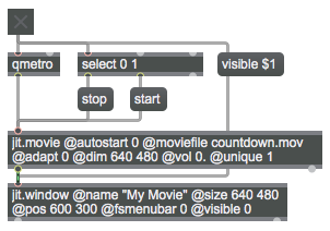
autostart / moviefile / adapt / dim / vol / unique
name / size / pos / fsmenubar / visible

autostart:
By default a jit.movie object’s ‘autostart’ attribute is set to 1, meaning that a movie (video file) will begin playing as soon as it’s loaded in. I usually prefer to have control of that myself, so I set the object’s ‘autostart’ attribute to 0 initially. That means I have to explicitly ‘start’ the movie when I want to view it. No problem. I use the 1 from the toggle object to trigger a ‘start’ message to the jit.movie object at the same time as I use it to turn on the qmetro. (If you don’t know what qmetro is, or why you should use it instead of metro, read about it in the example called “Simplest possible A-B video switcher” and in the article linked to on that page called “Event Priority in Max (Scheduler vs. Queue)”.)

moviefile:
Instead of reading a video file into jit.movie with a ‘read’ message, you can have it be read in automatically by specifying it with the ‘moviefile’ attribute. A couple of things to be aware of: 1) When you read a file in this way, jit.movie does not send out a ‘read’ message as described in the post “Detect when a movie has been read successfully“. So, if you’re relying on that message coming out to trigger other events in your patch, you need to read the movie in by sending a ‘read’ message to jit.movie (perhaps triggered by loadbang). 2) In Mac OS 10.8.5 or lower, there is a bug in jit.movie such that the ‘@autostart 0’ attribute setting described above will not work in conjunction with the ‘moviefile’ attribute unless it comes before the ‘moviefile’ attribute, as it does in this example patch. [I’ve reported the bug to Cycling ’74, so hopefully that second caveat will become obsolete soon.]

The next two attributes in the example show how you can force the matrix dimension of jit.movie to be something other than the size of the movie itself, if you want to. (For example, maybe the movie being read is higher-definition than you need, and you want to set a specific size of matrix to come out of jit.movie.) If you do that, the movie will be resized to fit the specified size of the object’s matrix. (Some pixels will be duplicated if the movie is being upsampled to fit in a larger matrix, and some pixels will be discarded if the movie is being downsampled to fit into a smaller matrix.)

adapt and dim:
The ‘adapt’ attribute determines whether the object’s matrix dimensions will be resized according to the dimensions of the video. By default, the ‘adapt’ attribute is on. If you want to enforce some other matrix size, you can set the ‘adapt’ attribute to 0 and use the ‘dim’ attribute to specify the width and height of the matrix.

vol:
In order to avoid any unwanted audio being played when the movie is read in, I like to have the movie’s audio volume (the ‘vol’ attribute) set to 0. You can then turn the audio up explicitly with a ‘vol’ message to jit.movie (not shown in this example). A ‘vol’ value of 1 is full volume, and values between 0 and 1 provide (logarithmically) scaled volume settings.

unique:
The ‘unique’ attribute, when turned on, means “Only send out a jit_matrix message if your matrix is different from the last time you sent it out.” If jit.movie gets a ‘bang’ message, but the content of its internal matrix is the same as the last time it got a ‘bang’, it won’t send anything out. Since jit.movie is constantly loading in new frames of video (assuming the video is running), if it’s getting a ‘bang’ message constantly it will report each new frame, but it won’t send out redundant messages. This is useful if the jit.movie will be receiving a lot of bangs but you only want it to send something out when it has some new content.

In this patch the qmetro will be sending out bangs constantly at its default interval of 5 ms, but because jit.movie‘s ‘unique’ attribute is turned on, it will only send out a ‘jit_matrix’ message each time it gets a unique frame of video. The result will be that the output of jit.movie (when the movie is running) will be at the frame rate, accurate to within 5 ms, which is accurate enough for our eyes. There will be quite a lot of unnecessary bangs sent to jit.movie, but it will ignore them if it has no new video content to send out.

That’s one way to handle the triggering of video frames, but it’s not the only way. Another way would be to query the frame rate of the movie with a ‘getfps’ message, which will cause jit.movie to send an ‘fps’ message out its right outlet reporting the frame rate of its video, and then use that fps value to calculate the desired interval for qmetro. With that method (1000./fps=interval), the qmetro would reliably send a bang at the frame rate of the video. If the playback rate of the video were to be changed with the ‘rate’ attribute, however, the qmetro would no longer be in sync with the rate at which new frames of video appear; in that case, the method shown in the example patch here might be more appropriate.

name:
The ‘name’ attribute of jit.window serves two purposes: 1) it shows in the title bar of the window, and 2) it’s the name that GL 3D animation objects in Jitter can refer to as their drawing location. For that second purpose, it’s most convenient for the name to be a single word; if you want a multi-word name, though, for the title bar of the window, you must put it in quotes so that Max will treat it as if it were a single word.

size and pos:
The ‘size’ and ‘pos’ attributes of jit.window set the dimensions of the window and its location on the screen. The two arguments of the ‘size’ attribute are the width and height of the window, in pixels. The two arguments of the ‘pos’ attribute are the horizontal and vertical offset of the top-left corner of the image from the top-left corner of the screen. So, in this patch, we’re specifying that we want the top-left corner of the image (the part of the window that does not include the title bar) to be located 600 pixels to the right and 300 pixels down from the top-left corner of the screen, and we want the image to be 640 pixels wide and 480 pixels high. The same result can be achieved with the ‘rect’ attribute, which lets you specify the left-top and bottom-right coordinates of the image onscreen; so in this example, the setting ‘@rect 600 300 1240 780’ would have the same effect.

fsmenubar:
The ‘fsmenubar’ attribute determines whether the menu bar should be shown when the window is put into ‘fullscreen’ mode. (Setting the ‘fsmenubar’ attribute to 1 means “Yes, I want the menu bar when I go to fullscreen,” and setting it to 0 means “No menubar when in fullscreen.”) Using the ‘fullscreen’ attribute to make the video fill the screen is not demonstrated in this patch, but is demonstrated well (and explained) in an example called “Using attributes to control video playback in Jitter” from the 2009 class. If I’m putting the window into ‘fullscreen’ mode, it’s usually because I want a nice presentation of video, so I usually don’t want the menubar to show then. But be careful; if you hide the menubar, how will you get out of fullscreen mode (with no menu commands available)? The 2009 example shows a good, standard way to solve that problem.

visible:
Using the ‘visible’ attribute of jit.window you can hide and show the window whenever you want. If there’s no reason for the user to see the window (e.g., if it’s just a blank screen) you might as well hide it, and then make it visible when you actually want to show video in it, as is done in this example.

The objects mtof and ftom provide easy conversion between MIDI pitch numbers and their equivalent equal-tempered frequency values. The purpose of this patch is just to show the conversion formulae that those objects use.

pitch-to-frequency conversion

The number of semitones of pitch difference from the base pitch of A above middle C is divided by 12 and used as a power of 2 by which to multiply the base frequency of 440 Hz. Thus, each semitone up from A is an additional twelfth root of two multiplication of the base frequency; each semitone downward is a negative twelfth root of two factor.

The expr object allows you to type in any mathematical expression, including some math functions not be found in other objects—e.g., log(), atan(), etc.—using a syntax that’s very similar to C programming language.

The timepoint object automatically and reliably sends out a ‘bang’ when the specified point in time is reached. How would you specify a point in time, and also make the notification “conditional”, such that it only occurs if a certain condition is met? This patch shows two different ways you might do that.

time point occurs if a condition is met

The method shown on the left is to have a timepoint object with no time specified. When the condition is met (the number 1 is received) the timepoint object receives a time specification. And if you want to cancel that, you can just set the timepoint to some time that will almost certainly never be reached.

The method shown on the right is to use a gate that can be conditionally opened (when the number 1 is received), and that is otherwise closed preventing the ‘bang’ from the timepoint from getting through.

Whenever the time interval of a metro object is specified using tempo-relative time units such as note values, the operation of that metro will be governed by the transport. The metro will only operate when the transport is turned on.

different metro behaviors

There are several ways to control the behavior of the metro via its attributes when it’s governed by the transport. Read in the manual about the @interval, @quantize, @active, @autostart, and @autostarttime attributes of metro.

The when object reports the current time of the transport. The timepoint object automatically reports when a specific moment in time has been reached.